28.22 Setting Output Width

REVIEW

# Load packages from the local library into the R session.

library(rattle)   # For the weatherAUS dataset.
library(ggplot2)  # To generate a density plot.

# Identify cities of interest.

cities <- c("Canberra", "Darwin", "Melbourne", "Sydney")

# Generate the plot.

weatherAUS %>%
  subset(Location %in% cities & ! is.na(Temp3pm)) %>%
  ggplot(aes(x=Temp3pm, colour=Location, fill=Location)) +
  geom_density(alpha=0.55)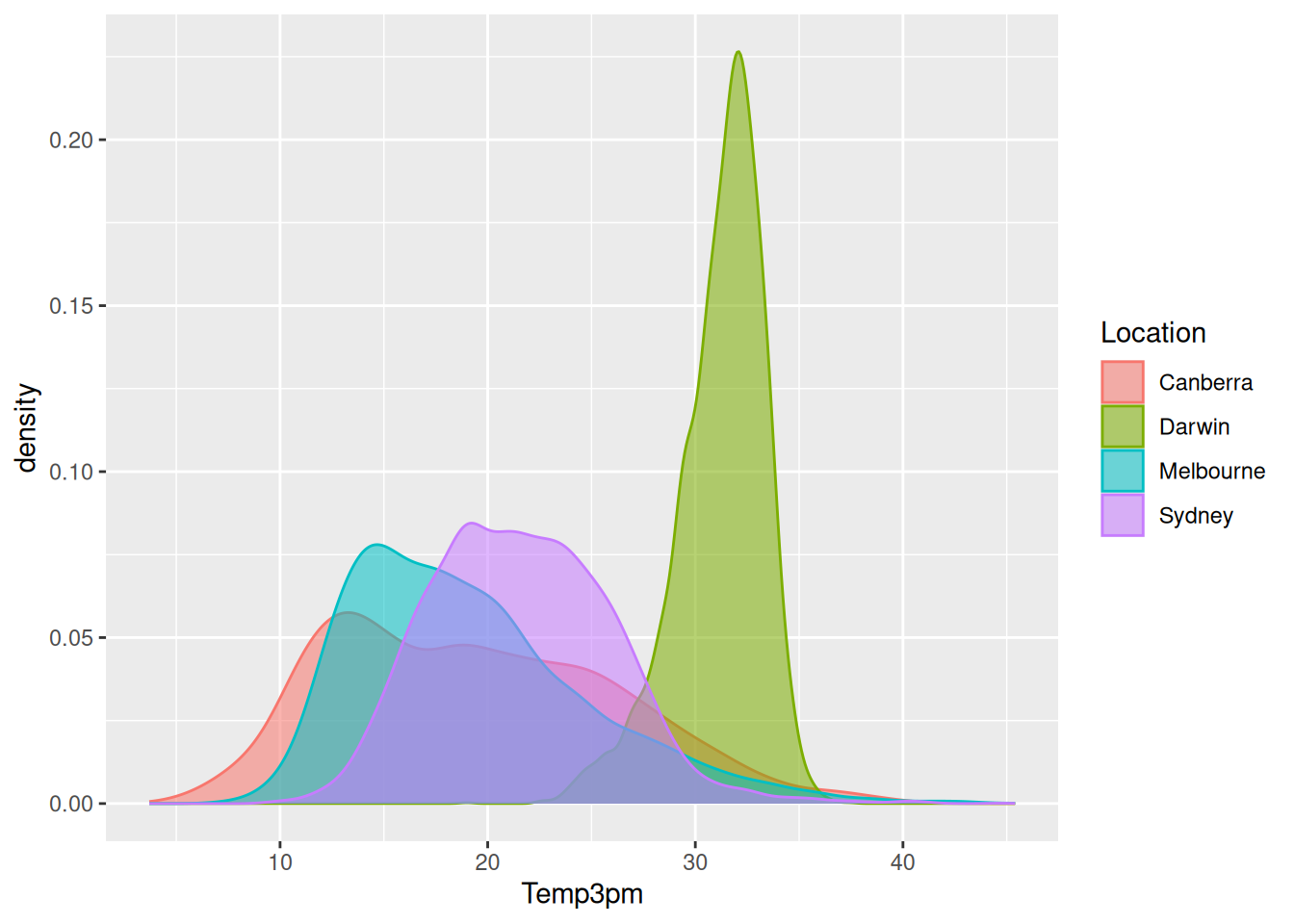

We can use the out.width= and out.height= to adjust how much space a figure takes up in the final document. The above figure is reduced to fill just half the textwidth of the document using:

<<myfigure, fig.align="center", fig.width=3.5, out.width="0.5\\textwidth"}
... R code ...
@

If that is too wide, we can reduce it to 90% of the page width with:

<<myfigure, fig.align="center", fig.width=3.5, out.width="0.9\\textwidth"}
... R code ...
@

# Load packages from the local library into the R session.

library(rattle)   # For the weatherAUS dataset.
library(ggplot2)  # To generate a density plot.

# Identify cities of interest.

cities <- c("Canberra", "Darwin", "Melbourne", "Sydney")

# Generate the plot.

weatherAUS %>%
  subset(Location %in% cities & ! is.na(Temp3pm)) %>%
  ggplot(aes(x=Temp3pm, colour=Location, fill=Location)) +
  geom_density(alpha=0.55)

---

Your donation will support ongoing availability and give you access to the PDF version of this book. Desktop Survival Guides include Data Science, GNU/Linux, and MLHub. Books available on Amazon include Data Mining with Rattle and Essentials of Data Science. Popular open source software includes rattle, wajig, and mlhub. Hosted by Togaware, a pioneer of free and open source software since 1984. Copyright © 1995-2022 Graham.Williams@togaware.com Creative Commons Attribution-ShareAlike 4.0