11.9 Bar Chart Faceted Background

20200823

ds %>%
  sample_frac(0.1) %T>%
  {assign("norain", . %>% select(-rain_tomorrow), 1)} %>%
  mutate(rain_tomorrow=factor(rain_tomorrow,
                              levels=(rain_tomorrow %>% unique() %>%
                                        sort() %>% rev()))) %>%
  ggplot(aes(x=wind_dir_3pm, fill=wind_dir_3pm)) +
  geom_bar(data=norain, fill="gray", alpha=0.5) +
  geom_bar() +
  facet_wrap(~ rain_tomorrow) +
  labs(x=vnames["wind_dir_3pm"], y="Count") +
  scale_y_continuous(labels=comma) +
  theme(legend.position="none")

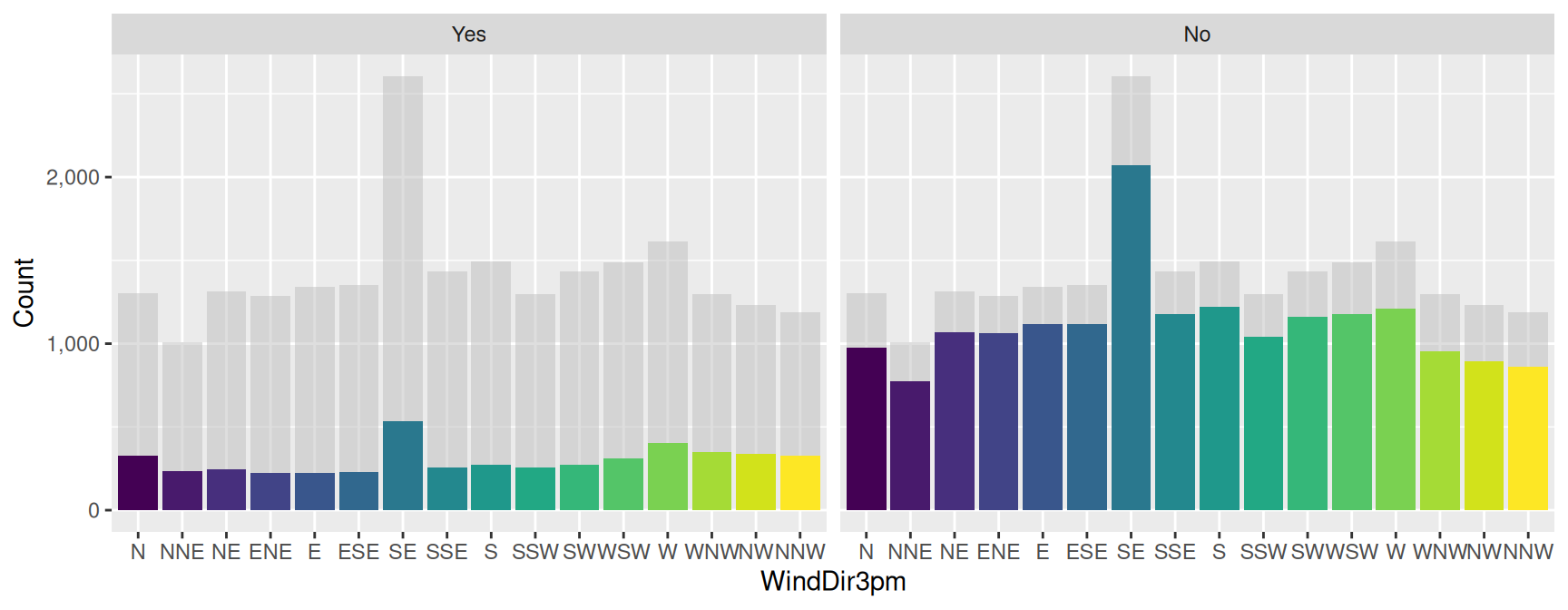
Using a faceted bar chart we can compare the individual charts with the global chart shown as a gray background.

Take a 10% sample. Remove the target column and save. Swap the order of No/Yes in the target column. Plot the wind direction. Add a grey layer with the non-target variable dataset. Add normal bar layer. Facet. Labels will have commas. Turn the legend off.

See https://drsimonj.svbtle.com/plotting-background-data-for-groups-with-ggplot2.

---

If you find this curated material useful then you can consider a donation to support it's ongoing availability and give you access to the PDF version of this book. The material has been scoped up by Generative AI without permission or any kind of recompense so do consider a donation if you can afford it. Unlike Generative AI your access to this materials is freely given. Desktop Survival Guides include Data Science, GNU/Linux, and MLHub. Books available on Amazon include Data Mining with Rattle and Essentials of Data Science. Togaware has a 30 year tradition of making popular open source software which includes sold privacy preserving productivity apps, rattle, wajig, and mlhub. Hosted by Togaware, a pioneer of free and open source software since 1984. Copyright © 1995-2022 Graham.Williams@togaware.com Creative Commons Attribution-ShareAlike 4.0