28.23 Add a Caption and Label

REVIEW

# Load packages from the local library into the R session.

library(rattle)   # For the weatherAUS dataset.
library(ggplot2)  # To generate a density plot.

# Identify cities of interest.

cities <- c("Canberra", "Darwin", "Melbourne", "Sydney")

# Generate the plot.

weatherAUS %>%
  subset(Location %in% cities & ! is.na(Temp3pm)) %>%
  ggplot(aes(x=Temp3pm, colour=Location, fill=Location)) +
  geom_density(alpha=0.55)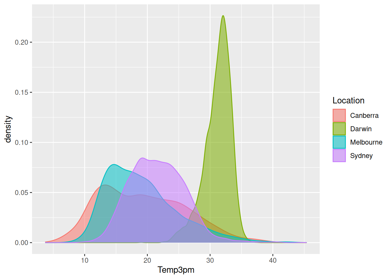

Adding a caption (which automatically also adds a label) is done using fig.cap=.

<<myfigure, fig.cap="The 3pm temperature for four locations.", fig.pos="h",...}
... R code ...
@

We have also used (but can’t see) fig.pos="h" which requests placement of the figure `here'' rather than letting it float. Other options are to place the figure at the top of a page (“t”), or the bottom of a page (“b”`). We can leave it empty and the placement is done automatically—that is, the figure floats to an appropriate location.

Once a caption is added, a label is also added to the figure so that it can be referred to in the document. The label is made up of fig: followed by the chunk label, which is myfigure in this example. So we can refer to the figure using \@ref(fig:myfigure) and \pageref{fig:myfigure}, which allows us to refer to Figure @ref(fig:knitr:myfigure_3pm_temp) on Page .

---

Your donation will support ongoing availability and give you access to the PDF version of this book. Desktop Survival Guides include Data Science, GNU/Linux, and MLHub. Books available on Amazon include Data Mining with Rattle and Essentials of Data Science. Popular open source software includes rattle, wajig, and mlhub. Hosted by Togaware, a pioneer of free and open source software since 1984. Copyright © 1995-2022 Graham.Williams@togaware.com Creative Commons Attribution-ShareAlike 4.0