11.33 Faceted Location Scatter Plot

REVIEW

ds %>%
  ggplot(aes(x=date, y=max_temp)) +
  geom_point(alpha=0.05, shape=".") +
  geom_smooth(method="gam", formula=y~s(x, bs="cs")) +
  facet_wrap(~location) +
  theme(axis.text.x=element_text(angle=45, hjust=1)) +
  labs(x=vnames["date"], y=vnames["max_temp"])

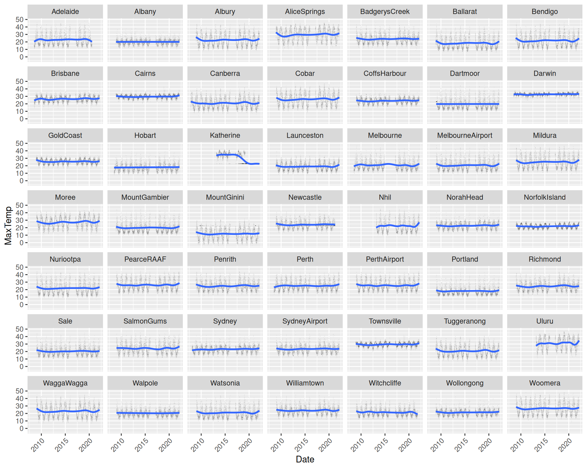
Partitioning the dataset by a categoric variable reduces the blob effect for big data. The plot uses location as the faceted variable to separately plot each location’s maximum temperature over time. Notice the seasonal effect across all plots, some with quite different patterns.

The plot uses ggplot2::facet_wrap() to separately plot each location. Using ggplot2::geom_point() with alpha= reduces the effect of overlaid points as does using smaller dots on the plots by way of shape=. Together this works to de-clutter the plot and improves the presentation with an emphasis on the patterns. The x-axis tick labels are rotated \(45^\circ\) using angle=45 within ggplot2::element_text() to avoid the labels overlapping. The hjust=1 forces the labels to be right justified.

---

If you find this curated material useful then you can consider a donation to support it's ongoing availability and give you access to the PDF version of this book. The material has been scoped up by Generative AI without permission or any kind of recompense so do consider a donation if you can afford it. Unlike Generative AI your access to this materials is freely given. Desktop Survival Guides include Data Science, GNU/Linux, and MLHub. Books available on Amazon include Data Mining with Rattle and Essentials of Data Science. Togaware has a 30 year tradition of making popular open source software which includes sold privacy preserving productivity apps, rattle, wajig, and mlhub. Hosted by Togaware, a pioneer of free and open source software since 1984. Copyright © 1995-2022 Graham.Williams@togaware.com Creative Commons Attribution-ShareAlike 4.0