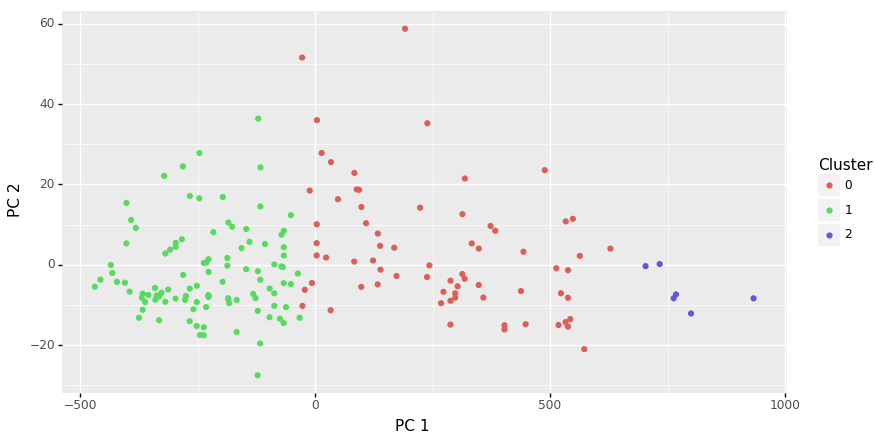
7.14 kmeans example wine dataset cluster

20220226

Now that we have a dataset in the right form we can train the k-means model. We’ll start with the original dataset before it was normalised.

ml train kmeans 3 wine.csv

alcohol,malic,ash,alcalinity,magnesium,total,flavanoids,nonflavanoid,proanthocyanins,color,hue,...
13.11,1.01,1.70,15.00,78.00,2.98,3.18,0.26,2.28,5.30,1.12,3.18,502.00,0
14.19,1.59,2.48,16.50,108.00,3.30,3.93,0.32,1.86,8.70,1.23,2.82,1680.00,1
13.88,1.89,2.59,15.00,101.00,3.25,3.56,0.17,1.70,5.43,0.88,3.56,1095.00,2

We can train and then use the model to predict and so doing extract the prediction for each observation into a file of just the cluster membership.

ml train kmeans 3 wine.csv |
  ml predict kmeans wine.csv |
  mlr --csv cut -f label > wine.pr

The original dataset has three classes so we might compare the clusters with the wine classes:

cat wine.data |
  cut -d"," -f 1 |
  awk 'NR==1{print "class"} {print}' |
  paste -d"," - wine.pr |
  sort |
  uniq -c

The pairwise count of the wine class and the clustering are reported. There is reasonable overlap. In this example the cluster labelled 0 covers much of the wine classes 2 and 3, whilst the cluster labelled 2 covers most of the wine class 1. There is then various “noise”.

 11 1,0
  6 1,1
 42 1,2
 69 2,0
  2 2,2
 48 3,0

Finally, we can visualise the multiple dimensional clustering using principle components:

cat wine.csv | 
    ml train kmeans 3 |
    ml predict kmeans wine.csv |
    ml visualise kmeans

---

Your donation will support ongoing availability and give you access to the PDF version of this book. Desktop Survival Guides include Data Science, GNU/Linux, and MLHub. Books available on Amazon include Data Mining with Rattle and Essentials of Data Science. Popular open source software includes rattle, wajig, and mlhub. Hosted by Togaware, a pioneer of free and open source software since 1984. Copyright © 1995-2022 Graham.Williams@togaware.com Creative Commons Attribution-ShareAlike 4.0